Comparing Economic Indicators in a Time-Series Chart
Time-series charts are useful for visualising how economic indicators change over time. By combining multiple series into one graph, we can compare their movements and identify periods in which they follow similar or contrasting trends.
In this example, we compare five indicators: the Reserve Bank of Australia’s cash rate, Australian inflation, the S&P 500, the Big Mac Index and the Australian dollar against the US dollar.
Preparing the data
Since the indicators are published at different frequencies and use different units of measurement, we need to organise the observations into half-yearly periods and standardise each variable to compare them consistently. Using the tempfile command, we create temorary files to store each prepared dataset until they are merged:
version 19.5

clear all

tempfile rate_old rate cpi stocks burger aud_old fx
Importing the RBA Interest Rate Data
We begin by importing two RBA datasets containing historical and recent cash rate targets. As the interest rates may be stored as text in one file and numeric values in the other, we first convert them into a consistent numeric format. We then use append to combine the datasets, followed by hofd() to assign each daily observation to its corresponding half-yearly period. The collapse (mean) command calculates the average cash rate for each period, while (count) records the number of available observations. Finally, isid checks that each half-year uniquely identifies an observation before the prepared dataset is saved:
import excel obsdate=A rba=B using "interest1.xls", ///
>     sheet("Data") cellrange(A12) clear

capture confirm string variable rba

if _rc == 0 {

else {

drop rba

rename rba_num rba

drop if missing(obsdate, rba)

keep if inrange(obsdate, td(01jan2000), td(31dec2010))

keep obsdate rba

confirm numeric variable rba

isid obsdate

save `rate_old'


import excel obsdate=A rba=B using "interest2.xlsx", ///
>     sheet("Data") cellrange(A12) clear

capture confirm string variable rba

if _rc == 0 {

else {

drop rba

rename rba_num rba

drop if missing(obsdate, rba)

keep if inrange(obsdate, td(01jan2011), td(31dec2026))

keep obsdate rba

confirm numeric variable rba

append using `rate_old'

isid obsdate

generate int halfyear = hofd(obsdate)

collapse (mean) rba (count) rba_days=rba, by(halfyear)

isid halfyear

save `rate'
Importing the Australian Inflation Data
Next, we import quarterly Consumer Price Index (CPI) data from the Australian Bureau of Statistics. Using qofd(), we create a quarterly time variable and declare the dataset as a time series with tsset. This allows us to calculate annual inflation using the L4. operator, which references the CPI index from four quarters earlier. We then calculate the average of the two quarterly annual inflation readings within each half-year:
import excel obsdate=A cpi_index=J using "inflation.xlsx", ///
>     sheet("Data1") cellrange(A11) clear

drop if missing(obsdate, cpi_index)

generate int quarter = qofd(obsdate)

isid quarter

tsset quarter, quarterly

generate double inflation = 100*(cpi_index/L4.cpi_index - 1)

generate int halfyear = hofd(obsdate)

keep if inrange(halfyear, yh(2000,1), yh(2026,2))

collapse (mean) inflation (count) inflation_quarters=inflation, by(halfyear)

isid halfyear

save `cpi'
This produces one representative annual inflation rate per half-year, rather than the percentage change occurring over those six months alone.
Importing the S&P 500 Data
The third dataset contains monthly S&P 500 index values. We import the CSV file using import delimited and convert its text dates into Stata dates using daily(). Following the same aggregation approach, we calculate the average of the six monthly index values within each half-year:
import delimited using "sp500.csv", varnames(1) case(lower) clear

generate double obsdate = daily(date, "YMD")

format obsdate %td

assert !missing(obsdate)

keep if inrange(obsdate, td(01jan2000), td(31dec2026))

drop if missing(sp500)

generate int halfyear = hofd(obsdate)

collapse (mean) sp500 (count) sp500_months=sp500, by(halfyear)

isid halfyear

save `stocks'
Importing the Big Mac Index Data
Next, we import the Big Mac Index published by The Economist, retaining only Australian observations using the country code AUS. The raw index values are converted into percentages, with positive and negative values indicating overvaluation and undervaluation of the Australian dollar under the index’s methodology. Unlike the previous indicators, the Big Mac Index was not consistently published twice yearly. We therefore use bysort to retain the latest observation within each half-year, leaving periods without published values as missing:
import delimited using "bigmac.csv", varnames(1) case(lower) clear

keep if iso_a3 == "AUS"

rename date date_string

generate double obsdate = daily(date_string, "YMD")

format obsdate %td

assert !missing(obsdate)

capture confirm numeric variable usd_raw

if _rc {

drop if missing(usd_raw)

generate double bigmac = 100*usd_raw

generate int halfyear = hofd(obsdate)

keep if inrange(halfyear, yh(2000,1), yh(2026,2))

bysort halfyear (obsdate): keep if _n == _N

keep halfyear bigmac

isid halfyear

save `burger'
Importing the AUD/USD Exchange Rate Data
Finally, we import the historical and recent AUD/USD exchange rate datasets, combining them using the same method as the RBA interest rate data. We then calculate the average exchange rate across each half-year:
import excel obsdate=A audusd=C using "aud1.xls", ///
>     sheet("Data") cellrange(A12) clear

drop if missing(obsdate, audusd)

keep if inrange(obsdate, td(01jan2000), td(31dec2009))

keep obsdate audusd

isid obsdate

save `aud_old'

import excel obsdate=A audusd=B using "aud2.xls", ///
>     sheet("Data") cellrange(A12) clear

drop if missing(obsdate, audusd)

keep if inrange(obsdate, td(01jan2010), td(31dec2026))

keep obsdate audusd

append using `aud_old'

isid obsdate

generate int halfyear = hofd(obsdate)

collapse (mean) audusd (count) aud_months=audusd, by(halfyear)

isid halfyear

save `fx'
Merging and Labelling the Data
With each indicator organised into half-yearly observations, we use merge 1:1 to combine the five datasets using their shared halfyear variable:
use `rate', clear

merge 1:1 halfyear using `cpi', nogen

merge 1:1 halfyear using `stocks', nogen

merge 1:1 halfyear using `burger', nogen

merge 1:1 halfyear using `fx', nogen

keep if inrange(halfyear, yh(2000,1), yh(2026,2))

format halfyear %th

sort halfyear

isid halfyear

tsset halfyear, halfyearly

tsfill

assert _N == 54

generate byte period_complete = ///
>     (rba_days > 0 & inflation_quarters == 2 & ///
>      sp500_months == 6 & aud_months == 6)
The tsset command declares the dataset as a half-yearly time series, while tsfill ensures all 54 periods are represented. We also create period_complete to identify complete reporting periods. Next, we assign descriptive labels to make the variables easier to interpret:
label variable halfyear "Half-year"

label variable rba "RBA cash rate target (%)"

label variable inflation "Annual CPI inflation (%)"

label variable sp500 "S&P 500 index (half-year mean)"

label variable bigmac "Australian Big Mac raw index (%)"

label variable audusd "AUD/USD exchange rate"

label variable period_complete "Full six-month reporting period"

label variable rba_days "RBA cash-rate observations"

label variable inflation_quarters "CPI annual-inflation readings"

label variable sp500_months "S&P 500 monthly observations"

label variable aud_months "AUD/USD monthly observations"
Standardising the Data
Since the five indicators use different units, we standardise them using egen with the std() function. This converts their values into z-scores, allowing them to be compared on a common scale. A foreach loop applies the calculation to all five variables, excluding incomplete reporting periods:
foreach var in rba inflation sp500 bigmac audusd {
We then inspect the combined dataset using list, check for missing values with misstable summarize, and save the results in Stata and CSV formats:
sort halfyear

list halfyear rba inflation sp500 bigmac audusd ///
>     period_complete, noobs sep(0)

list halfyear if missing(bigmac), noobs

misstable summarize rba inflation sp500 bigmac audusd

tabulate period_complete

save "economic_indicators_2000_2026.dta", replace

export delimited using "economic_indicators_2000_2026.csv", replace
Creating the Chart
Finally, we use twoway to display all five standardised indicators on one time-series chart. First, we create horizontal-axis labels showing each calendar year rather than the half-yearly date format:
local xlabels

forvalues year = 2000/2026 {
We then overlay five line plots, assigning each indicator a different colour and adding a legend to identify them:
twoway ///
>     (line z_rba halfyear, ///
>         sort cmissing(n) lcolor(navy) lwidth(medthick)) ///
>     (line z_inflation halfyear, ///
>         sort cmissing(n) lcolor(maroon) lwidth(medthick)) ///
>     (line z_sp500 halfyear, ///
>         sort cmissing(n) lcolor(forest_green) lwidth(medthick)) ///
>     (line z_bigmac halfyear, ///
>                 sort cmissing(y) lcolor(orange) lwidth(medthick)) ///
>     (line z_audusd halfyear, ///
>         sort cmissing(n) lcolor(purple) lwidth(medthick)), ///
>     title("Comparing Five Economic Indicators") ///
>     xtitle("Year") ///
>     ytitle("Standardised value") ///
>     xlabel(`xlabels', angle(45) labsize(small)) ///
>     yline(0, lpattern(dash) lcolor(gs12)) ///
>     legend(order(1 "RBA interest rate" ///
>                  2 "Australian inflation" ///
>                  3 "S&P 500" ///
>                  4 "Big Mac Index" ///
>                  5 "AUD/USD") ///
>            position(6) rows(2) size(small)) ///
>     graphregion(color(white)) ///
>         name(comparison)
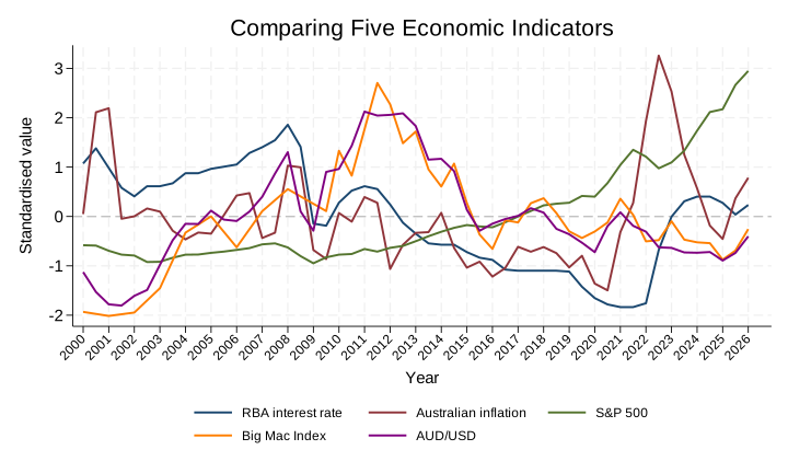
The sort option connects observations chronologically, while cmissing(y) joins the Big Mac Index line across periods without published values. The yline(0) option adds a reference line representing the average standardised value.
Summary
The completed chart compares five economic indicators across 27 years, allowing us to identify periods of economic change and observe similarities or differences in their movements. Because the variables are standardised, the lines represent values relative to each indicator’s historical average rather than their original units.