A Scatter Plot in Stata with Reduced Noise

You can use the binscatter command in Stata to create a scatter plot where the values are separated into bins (similar to a histogram). By placing individual values into bins that each represent a range of values, it allows trends in a scatter plot to be more easily seen and interpretable. The binscatter command also allows you to apply predictive lines (such as linear or quadratic) more easily than a regular scatter. Use the linetype() option with either lfit for linear, qfit for quadratic, or connect to run a line connecting the dots.

To create a binned scatter in Stata, you first need to download the binscatter command from the SSC. You do this in Stata with the following command:

ssc install binscatter

To generate this graph in Stata, use the following commands:

sysuse nlsw88, clear
binscatter wage tenure, linetype(qfit)

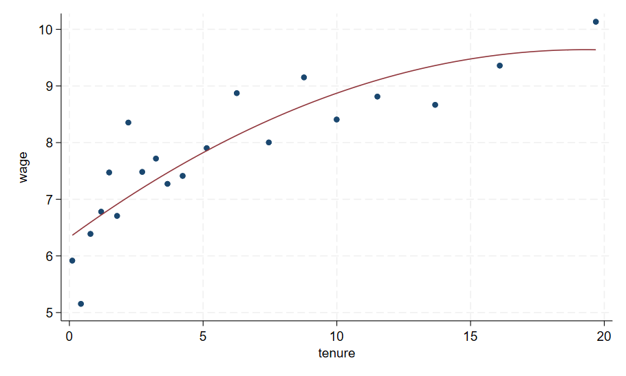
Let’s compare this with the original scatter:

To generate this comparison in Stata, use the following commands:

sysuse nlsw88, clear
scatter wage tenure, title(Normal Scatter) name(g1, replace) || qfit wage tenure, legend(off) graphregion(fcolor(white))
binscatter wage tenure, linetype(qfit) title(Bin Scatter) name(g2, replace)
graph combine g1 g2