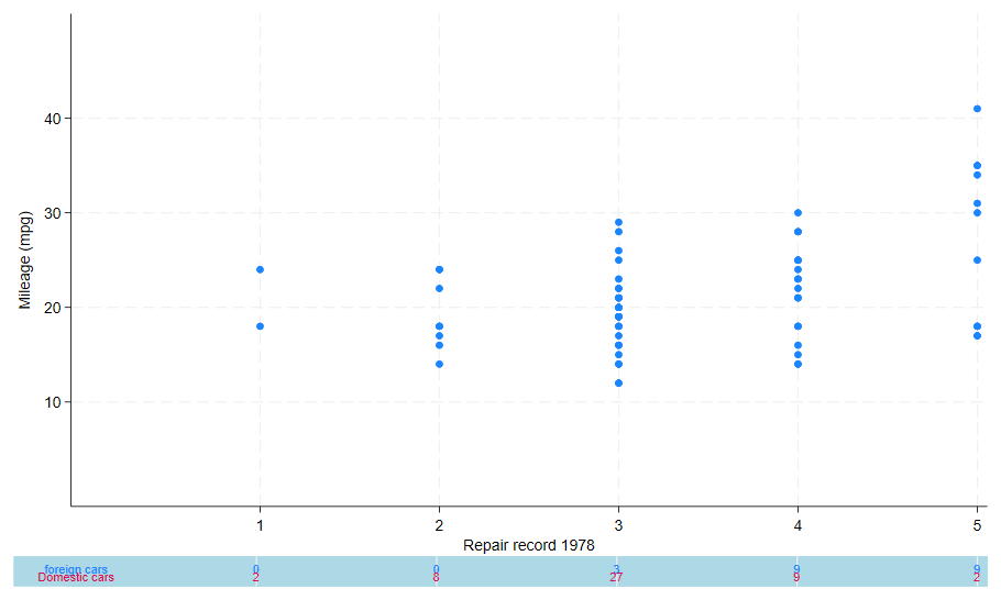
Add a Table to the Bottom of your Graph

You can add a simple table to the bottom of your graph. To do this you create the table by adding extra blank “observations” to the end of your dataset for each row of the table you want. You can then “graph” the table and combine it at the bottom of the first graph.

To generate this graph in Stata, use the following commands:

sysuse auto, clear
 
scatter mpg rep78, yscale(range(0 50)) , ysize(2) name(g1, replace) xlabel(1(1)5)
 
contract rep78 foreign
fillin rep78 foreign
replace _freq=0 if missing(_freq)
 
set obs `=_N + 2'
 
tostring _freq, replace
replace rep78=0 in `=_N - 1'
replace rep78=0 in `=_N'
replace foreign=1 in `=_N - 1'
replace foreign=0 in `=_N'
 
replace _freq = "foreign cars " in `=_N - 1'
replace _freq = "Domestic cars" in `=_N'
 
scatter foreign rep78 if foreign == 1, mlabel(_freq) msymbol(none) mlabgap(-2) mlabposition(12) || scatter foreign rep78 if foreign == 0, mlabel(_freq) msymbol(none) mlabgap(-2) mlabposition(6) name(g2, replace) legend(off) ytitle("b") fysize(5) xscale( off) yscale( off fill) graphregion(color(ltblue )) plotregion(color(ltblue )) ylabel(,nogrid) xlabel( 1(1)5 )
 
graph combine g1 g2, cols(1) xcommon imargin(0 0 0 0)