Geospatial analysis in Stata: Mapping multiple variables
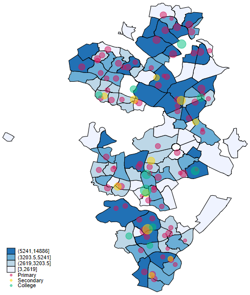
Above is a map showing the population density of suburbs in ACT, combined with ACT public school locations and population sizes. The different point sizes represent different school sizes. Today I’m going to show you how to create the above graph in Stata.
In order to draw the map, we need information from a variety of datasets. All the datasets are downloadable from ACT government open data portal. I have prepared the data and distilled it into the three Stata datasets we will need to create the map above. However, if you want to know how to do this yourself, the following datasets were downloaded and modified:
-
The ACT map shape files were downloaded directly from here. However, if this link does not work you can navigate to this link from here. You only need the SHP and DBF files. Once downloaded, you will need to convert to Stata map files using the spshape2dta command, and then you will need to remove districts so you only have suburbs. This is not entirely necessary but it does make the map more discernable, as the lower half of the ACT does not contain any schools.
-
The ACT population data can be found here. It is separated by year, age range, and gender, so you will need to perform some data management to get the overall population data. To get the latest data, remove all but the latest year, and remove the two genders so you are left with “Persons” only which is a combined total. You will then need to add all the age ranges together for each suburb to get a combined total.
-
The ACT school location data can be found here. Each layer needs to be downloaded separately. Please note, the school geographic data does not use the same geographical coordinate system as the ACT map shape files. You will need to convert either the ACT map shape files, or the school shape files, to the other system. It is advisable to convert the ACT map shape files from the GEOGCS GDA2020 degree-decimal system to the WGS 1984 Web Mercator Auxiliary Sphere system (used by the school files), as this way you only need to convert one map. For my datasets I converted all the school files to the GDA2020 degree-decimal system purely because I prefer this system, but it is easier to go the other way. I used the program MapWindow5 to convert my map files from one system to the other. You can download this program here.
-
The ACT public school size data can be found here Choose Census - All ACT Schools. Then download word version of Census of ACT Public Schools August CURRENT_YEAR. The data you need is in a bunch of tables that can be copied directly into the Stata Data Editor. You will need to perform some data management to get the dataset into the correct format.
I have pre-prepared all the data we need and distilled it into the three datasets needed to create our map. The steps I followed to prepare the data are as follows:
- Used the spshape2dta command to convert the ACT map shape files to a Stata spatial dataset.
- Loaded the map file, checked it was appropriately link with the corresponding _shp.dta file with the spset command, and then removed any observations that were not suburbs (e.g. districts etc.) and saved the map file.
- Loaded the population file, dropped all but the latest year, dropped all genders except “Persons”, used the egen command with the total option to create a new variable that totalled the population by suburb. Kept only one age range as I now had the total. Saved the dataset.
- Loaded the map file again, merged the population file into the map file by suburb using frames, frlink, and frget. Checked for any issues with mismatched suburb names, fixed and re-merged, then saved the map file again.
- Downloaded each school location map file, loaded it into MapWindow5, converted it to the GEOGCS GDA2020 degree-decimal coordinate system, and exported it.
- Used the spshape2dta command to convert each school location map to a Stata spatial dataset, then appended all the regular map dta files together, and separately appended all the _shp map dta files together. Saved both sets separately.
- Copied the ACT school size data into Stata and edited it so it would match the school location map files.
- Used frames, frlink, and frget to merge the ACT school size data into the ACT school location map dataset, then saved it.
At the end of this process, I have three datasets:
So now we have all the data ready to draw the map! Let’s start the journey.
First, download the three Stata datasets shown above and put them in your current working directory. If you do not know what folder your current working directory is, it is shown in the bottom-left corner of your Stata. Alternatively, you can use the pwd command to print your current working directory to the results pane in Stata.
Once you have your three datasets in your current working directory, you need to spset the schools.dta dataset and link it with the schools_shp.dta dataset. You do this with the following commands:
use act_suburbs_pop.dta
spset
spset, shpfile(act_suburbs_shp.dta) modify

The spset command by itself should tell you if the dataset is recognised as a spatial dataset. I run this before linking the shapefile to confirm that the act_suburbs_pop.dta dataset is a spatial dataset, otherwise the second spset command that adds the shapefile will not work.
NOTE: Ordinarily, if you are creating a spatial dataset directly from SHP and DBF files using the spshape2dta command then you will not need to attach a shapefile in this way. However, because I have done this step for you and am sharing the result with you, these files need to be unlinked when shared and then re-linked when downloaded.
You can now draw an initial blank map of school districts as follows:
grmap, activate
grmap
NOTE: The grmap, activate command is needed to initialize Stata’s mapping functions if you have never used them before. Once you have done this once, it does not need to be repeated.
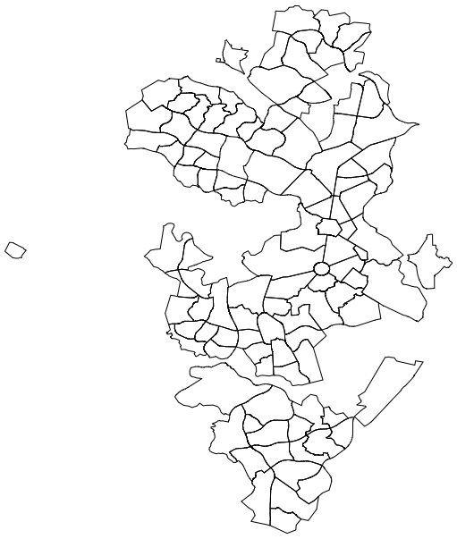
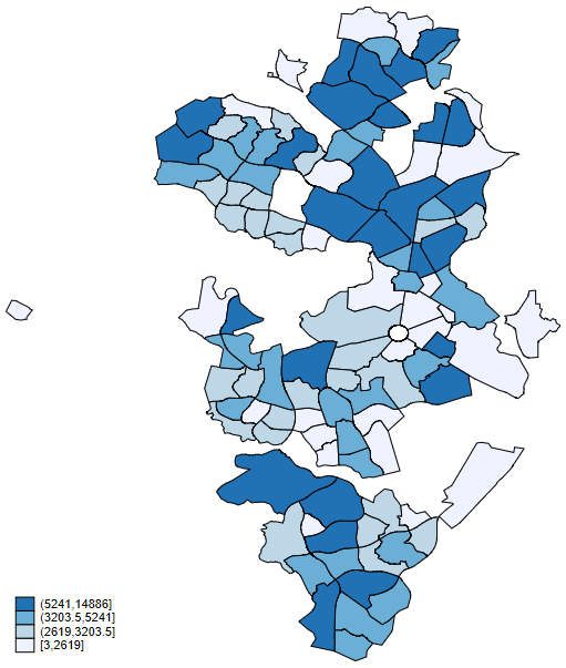
Since I have already merged the ACT population data into the dataset for you, you can also draw an initial choropleth map using the following command:
grmap population
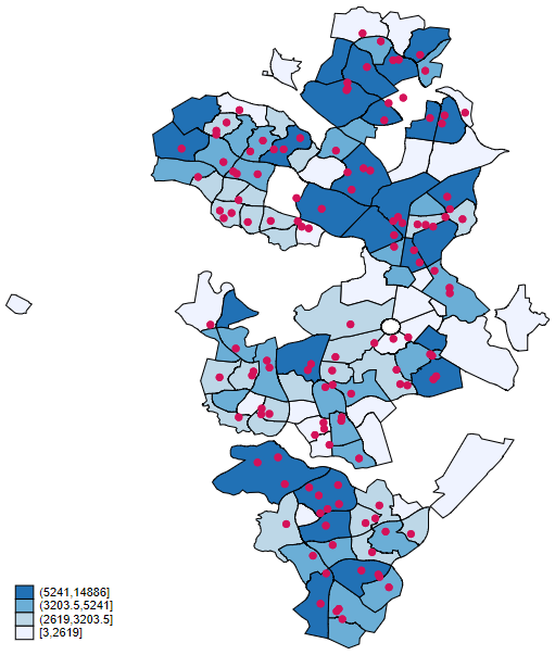
Now we have our ACT map data with population by suburb, we can add our school_pop_loc.dta data in as point data to show the location of all schools on our choropleth map. To start, I am just going to display all the schools in the ACT.
grmap population, point(data(school_pop_loc.dta) xcoord(_CX) ycoord(_CY) size(small) fcolor(stc2))
The initial map showed only ACT schools that fit perfectly into three categories: Primary (P-6 or K-6); Secondary/High (7-10); and College (11-12). Most private or non-government schools do not fit these categories and there are even some public schools that don’t fit because they are combined. So we need to eliminate these from our map using the select() suboption within the point() option. Additionally, to separate by categories on the map we need to add the by() suboption to the point() option. The command is as follows:
grmap population, point(data(school_pop_loc.dta) xcoord(_CX) ycoord(_CY) select(drop if type_simple == 4) by(type_simple) size(small small small) fcolor(stc2 stc4 stc3) legenda(on))
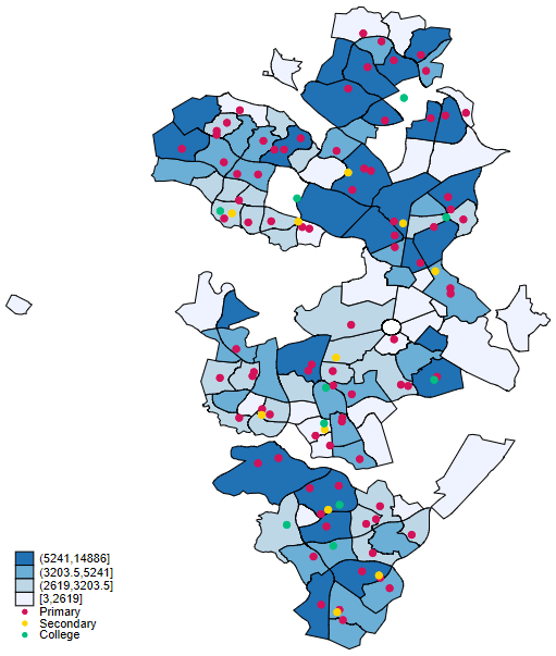
For the command, you need to understand exactly how many categories are going to be displayed from your point dataset, because you will need to specify that number of sizes and that number of colours. For example in our map above I have three school categories, so I specified the small size three times and I specified three different colours for each category.
Our final step is to change the size of the points based on the size of the schools. There are four population variables in the point dataset. The first three population variables contain the population for each category (Primary/Secondary/College) and the fourth category is the total. The populations are separated in this way to accommodate schools where more than one category of students is represented, so you can display populations in different ways on the map. To start we will just use the total population variable schpoptot, because we are only mapping schools that fit perfectly into the three categories.
grmap population, point(data(school_pop_loc.dta) xcoord(_CX) ycoord(_CY) select(drop if type_simple == 4) by(type_simple) proportional(schpoptot) size(small small small) fcolor(stc2%50 stc4%50 stc3%50) legenda(on))

The proportional() suboption of the point() option sizes the school points based on their population size. You will notice I have added %50 to each of the three colours. This is because when shown proportionally some of the school points overlap or are completely engulfed, and so I have added transparency to still be able to fully appreciate the data.
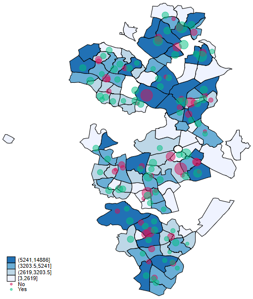
There are other maps you could create with this data. For example, perhaps I want to look at the difference between populations of public versus private/non-government schools. I would do this with the following command:
grmap population, point(data(school_pop_loc.dta) xcoord(_CX) ycoord(_CY) by(state) proportional(schpoptot) size(small small) fcolor(stc2%50 stc3%50) legenda(on))
If you have any questions, please feel free to contact us at sales@surveydesign.com.au. We would be happy to answer any of your questions.